Notifications
ALL BUSINESS
COMIDA
DIRECTORIES
ENTERTAINMENT
FINER THINGS
HEALTH
MARKETPLACE
MEMBER's ONLY
MONEY MATTER$
MOTIVATIONAL
NEWS & WEATHER
TECHNOLOGIA
TV NETWORKS
VIDEOS
VOTE USA 2026/2028
INVESTOR RELATIONS
COMING 2026 / 2027
ALL BUSINESS
COMIDA
DIRECTORIES
ENTERTAINMENT
FINER THINGS
HEALTH
MARKETPLACE
MEMBER's ONLY
MONEY MATTER$
MOTIVATIONAL
NEWS & WEATHER
TECHNOLOGIA
TV NETWORKS
VIDEOS
VOTE USA 2026/2028
INVESTOR RELATIONS
COMING 2026 / 2027
About Me
 Latinos Media
 Latinos Media provides all types of news feeds on a daily basis to our Members
Posted by - Latinos Media -
on - February 11, 2024 -
Filed in - Weather -
-
740 Views - 0 Comments - 0 Likes - 0 Reviews
Since the blogosphere continues to amplify Gavin Schmidt’s claim that the way John Christy and I plot temperature time series data is some form of “trickery”, I have come up with a way to demonstrate its superiority. Following a suggestion by Heritage Foundation chief statistician Kevin Dayaratna, I will do this using only climate model data, and not comparing the models to observations. That way, no one can claim I am displaying the data in such a way to make the models “look bad”.
The goal here is to plot multiple temperature time series on a single graph in such a way the their different rates of long-term warming (usually measured by linear warming trends) are best reflected by their placement on the graph, without hiding those differences.
A. Raw Temperatures
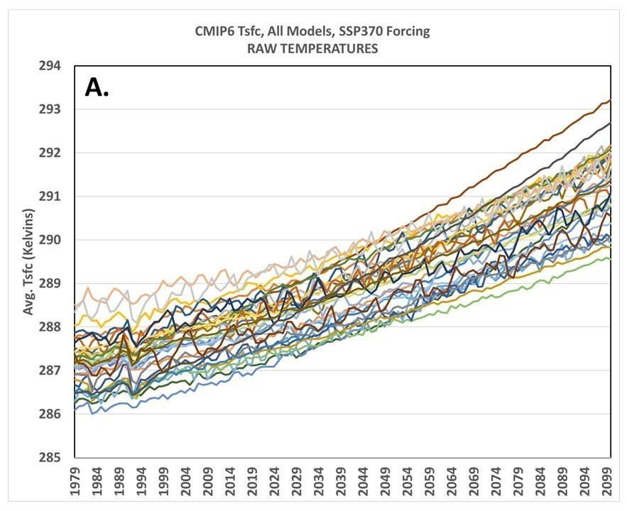
Let’s start with 32 CMIP6 climate model projections of global annual average surface air temperature for the period 1979 through 2100 (Plot A) and for which we have equilibrium climate sensitivity (ECS) estimates (I’ve omitted 2 of the 3 Canadian model simulations, which produce the most warming and are virtually the same).
Here, I am using the raw temperatures out of the models (not anomalies). As can be seen in Plot A, there are rather large biases between models which tend to obscure which models warm the most and which warm the least.

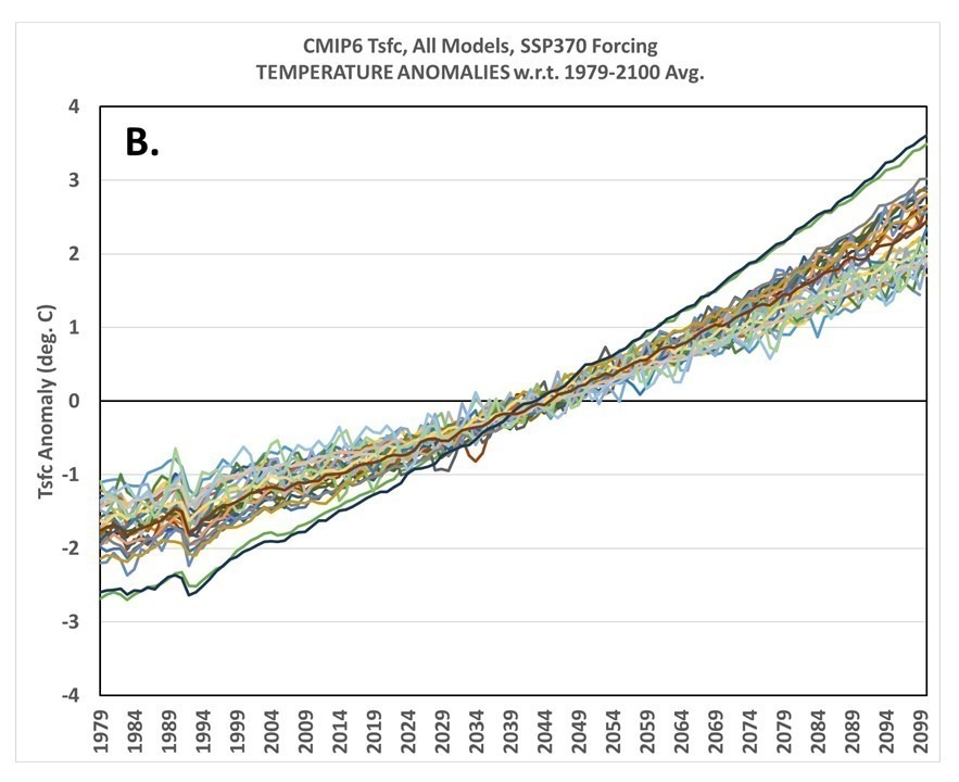
B. Temperature Anomalies Relative to the Full Period (1979-2100)
Next, if we plot the departures of each model’s temperature from the full-period (1979-2100) average, we see in Plot B that the discrepancies between models warming rates are divided between the first and second half of the record, with the warmest models by 2100 having the coolest temperature anomalies in 1979, and the coolest models in 2100 having the warmest temperatures in 1979. Clearly, this isn’t much of an improvement, especially if one wants to compare the models early in the record… right?
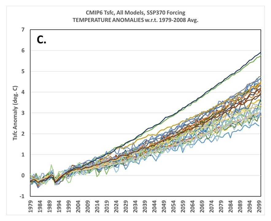
C. Temperature Anomalies Relative to the First 30 Years
The first level of real improvement we get is by plotting the temperatures relative to the average of the first part of the record, in this case I will use 1979-2008 (Plot C). This appears to be the method favored by Gavin Schmidt, and just looking at the graph might lead one to believe this is sufficient. (As we shall see, though, there is a way to quantify how well these plots convey information about the various models’ rates of warming.)
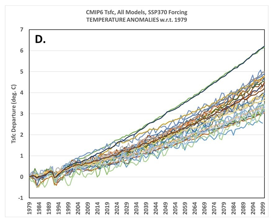
D. Temperature Departures from 1979
For purposes of demonstration (and since someone will ask anyway), let’s look at the graph when the model data are plotted as departures from the 1st year, 1979 (Plot D). This also looks pretty good, but if you think about it the trouble one could run into is that in one model there might be a warm El Nino going on in 1979, while in another model a cool La Nina might be occurring. Using just the first year (1979) as a “baseline” will then produce small model-dependent biases in all post-1979 years seen in Plot D. Nevertheless, Plots C and D “look” pretty good, right? Well, as I will soon show, there is a way to “score” them.
E. Temperature Departures from Linear Trends (relative to the trend Y-intercepts in 1979)
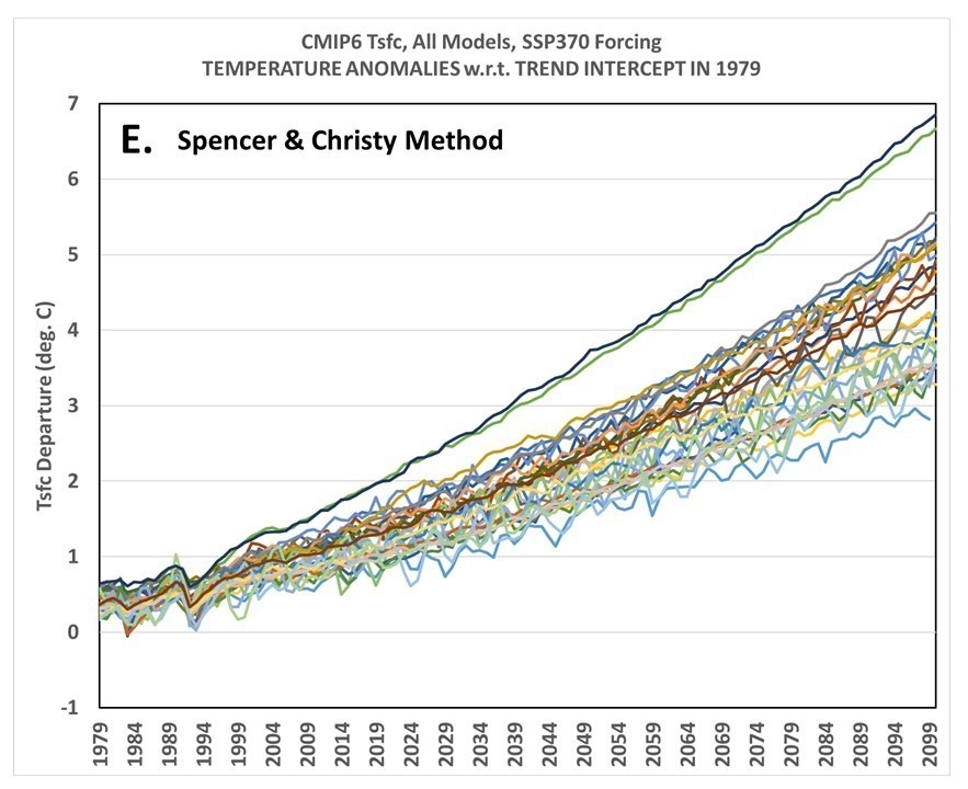
Finally, I show the method John Christy and I have been using for quite a few years now, which is to align the time series such that their linear trends all intersect in the first year, here 1979 (Plot E). I’ve previously discussed why this ‘seems’ the most logical method, but clearly not everyone is convinced.
Admittedly, Plots C, D, and E all look quite similar… so how to know which (if any) is best?
How the Models’ Temperature Metrics Compare to their Equilibrium Climate Sensitivities
What we want is a method of graphing where the model differences in long-term warming rates show up as early as possible in the record. For example, imagine you are looking at a specific year, say 1990… we want a way to display the model temperature differences in that year that have some relationship to the models’ long-term rates of warming.
Of course, each model already has a metric of how much warming it produces, through their diagnosed equilibrium (or effective) climate sensitivities, ECS. So, all we have to do is, in each separate year, correlate the model temperature metrics in Plots A, B, C, D, and E with the models’ ECS values (see plot, below).
When we do this ‘scoring’ we find that our method of plotting the data clearly has the highest correlations between temperature and ECS early in the record.
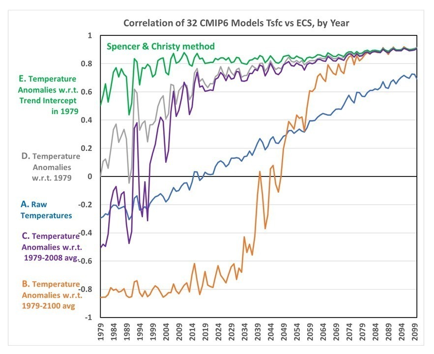
I hope this is sufficient evidence of the superiority of our way of plotting different time series when the intent is to reveal differences in long-term trends, rather than hide those differences.
The post Proof that the Spencer & Christy Method of Plotting Temperature Time Series is Best first appeared on Roy Spencer, PhD..